1.9 Representing Texts as Vectors: TF-IDF
Contents
1.9 Representing Texts as Vectors: TF-IDF#
In the lesson about making a search engine over Medium with bag of words, we saw that some words are somewhat more important than others when computing article scores with respect to the query. Indeed, we heuristically noticed that ignoring stopwords (i.e. giving them a weight of zero, while giving a unitary weight to all the other tokens) results in a better search engine.
In this lesson, we learn about another heuristic that assigns different weights to tokens and often results in better search engines, namely TF-IDF.
Zipf’s Law#
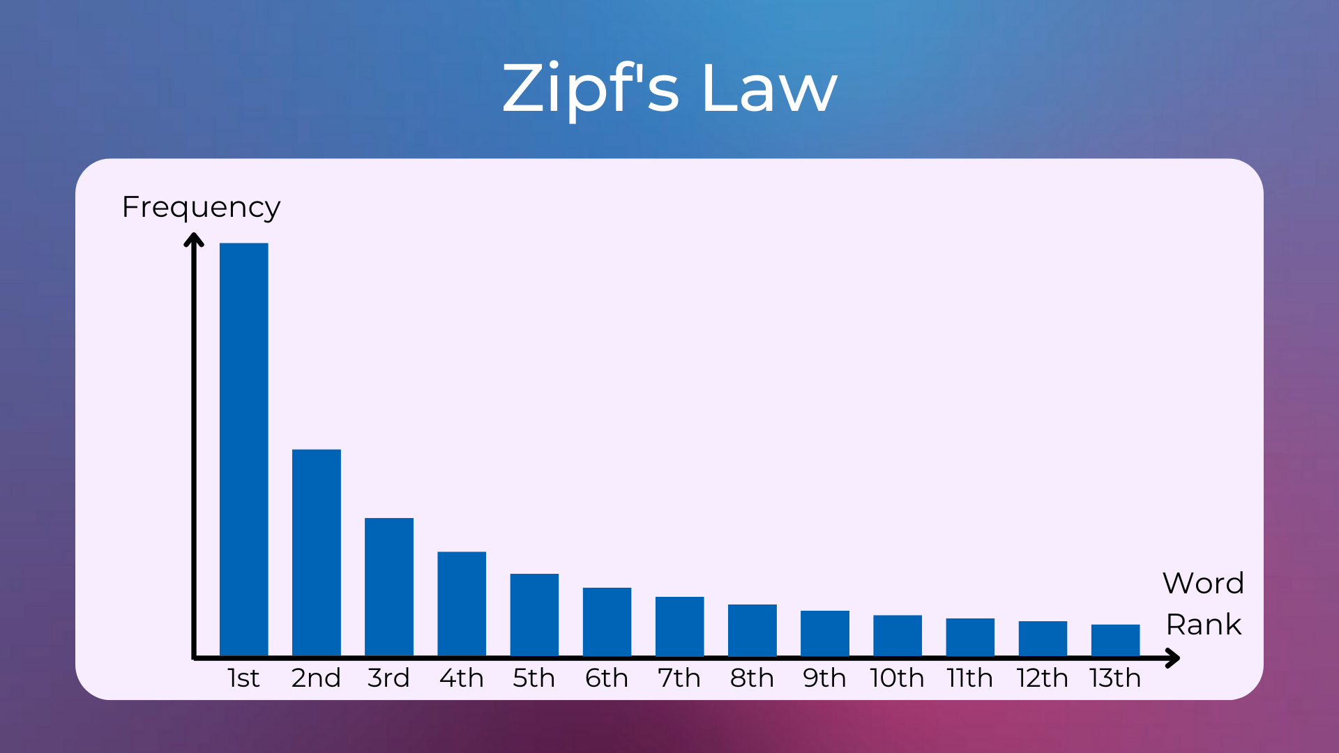
First, let’s notice that words are typically distributed in languages according to a power law called Zipf’s law. Here’s how Wikipedia describes it.
Zipf’s law was originally formulated in terms of quantitative linguistics, stating that given some corpus of natural language utterances, the frequency of any word is inversely proportional to its rank in the frequency table. […] For example, in the Brown Corpus of American English text, the word “the” is the most frequently occurring word, and by itself accounts for nearly 7% of all word occurrences. True to Zipf’s Law, the second-place word “of” accounts for slightly over 3.5% of words […]. Only 135 vocabulary items are needed to account for half the Brown Corpus.
So, this is what the distribution of the frequencies of the words in a corpus should look like.
Let’s quickly verify if this distribution holds also for the dataset of Medium articles that we used in the last projects.
Zipf’s Law in Medium Articles#
Let’s import the necessary libraries. The only different library from the ones in the previous lessons is plotly, which is a data visualization library for making beautiful interactive plots.
from huggingface_hub import hf_hub_download
import nltk
nltk.download('punkt')
from nltk.tokenize import word_tokenize

import pandas as pd
import plotly.express as px

from collections import Counter
import re
We then download the dataset of Medium articles from the Hugging Face Hub and convert it to a pandas dataframe.
# download dataset of Medium articles from
# https://huggingface.co/datasets/fabiochiu/medium-articles
df_articles = pd.read_csv(
  hf_hub_download("fabiochiu/medium-articles", repo_type="dataset", filename="medium_articles.csv")
)

# There are 192,368 articles in total, but let's sample only 30,000 of them to
# make computations faster
df_articles = df_articles.sample(n=30000)

df_articles.head()
| title | text | url | authors | timestamp | tags | |
|---|---|---|---|---|---|---|
| 0 | What if Robots Take Over the World | Image Courtesy: Unsplash.com\n\nYou might have... | https://medium.com/@minisculestories/what-if-r... | ['Miniscule Stories'] | 2020-12-05 19:35:52.037000+00:00 | ['Robots'] |
| 1 | Spice It Up With Language Honey | Spice It Up With Language Honey\n\nPhoto by An... | https://2madness.com/spice-it-up-with-language... | ['Jodi Urgitus'] | 2020-09-16 01:59:13.972000+00:00 | ['Millennials', 'Language', 'Exercise', 'Lifes... |
| 2 | How NOT to get scammed on the Internet | I have an interesting story for you to read. J... | https://medium.com/@angeliichoo77/how-not-to-g... | [] | 2020-12-14 01:13:46.746000+00:00 | ['Scam', 'Online Safety', 'Online Shopping', '... |
| 3 | Three months dating an Artificial ‘almost’ Int... | Three months dating an Artificial ‘almost’ Int... | https://medium.com/q-n-english/three-months-da... | [] | 2017-11-29 12:21:28.429000+00:00 | ['AI', 'Voice Assistant', 'Qnenglish', 'Amazon... |
| 4 | Streaming Payments and the Future of Interoper... | Talk given by Evan Schwartz\n\nEvan Schwartz i... | https://medium.com/mitbitcoinclub/streaming-pa... | ['Sathya Peri'] | 2018-05-10 21:45:37.760000+00:00 | ['Blockchain', 'Altcoins', 'Cryptocurrency', '... |
Next, let’s do some simple text preprocessing and count how many occurrences we have for each token in the whole dataset.
def from_text_to_counter(full_text):
  # convert texts to lowercase
  full_text_lower = full_text.lower()

  # remove punctuation from articles
  full_text_no_punctuation = re.sub(r'[^\w\s]', ' ', full_text_lower)

  # tokenize texts
  full_text_tokenized = word_tokenize(full_text_no_punctuation)

  # count the occurrences of each token
  token_counter = Counter(full_text_tokenized)

  return token_counter

# count the occurrences of each token
full_text = " ".join(df_articles["text"].values)
token_counter = from_text_to_counter(full_text)
We are now ready to plot the number of occurrences of the most frequent tokens in the dataset.
# get occurrences of top 30 tokens
top_n = 30
xs, ys = list(zip(*token_counter.most_common(top_n)))

# plot
plot_title = "Tokens and their occurrencies on the Medium dataset"
labels = {
  "x": "Tokens",
  "y": "Number of occurrencies"
}
fig = px.bar(x=xs, y=ys, template="plotly_dark", title=plot_title, labels=labels)
fig.show()
As expected, the most common tokens are prepositions and articles such as “the”, “to”, and “and”. Let’s see if their occurrences are approximately inversely proportional to their rank.
# get occurrences of top 30 tokens
top_n = 30
xs, ys = list(zip(*token_counter.most_common(top_n)))

# get zipf values of top 30 occurrences
ys_zipfs = [ys[0]]
for i in range(1, len(ys)):
  new_value = (ys_zipfs[0] / (i + 1))
  ys_zipfs.append(new_value)

# plot
plot_title = "Tokens and their occurrencies on the Medium dataset (red) VS Zipf's law (blue)"
labels = {
  "x": "Tokens",
  "y": "Number of occurrencies"
}
fig = px.line(x=xs, y=ys_zipfs, template="plotly_dark", title=plot_title, labels=labels)
fig.add_bar(x=xs, y=ys)
fig.update_layout(showlegend=False)
fig.show()
It looks like there are some differences between the values predicted by the Zipf’s law and the number of occurrences in the Medium dataset, maybe because articles on Medium don’t properly represent common English usage such as in the Brown Corpus.
Zipf’s Law in Brown Corpus#
Let’s try doing the same with the texts available in nltk from the Brown Corpus.
import nltk
nltk.download('gutenberg')
We then download all the corpora and count the occurrences of each token.
# list of Shakespeare corpora
file_ids = nltk.corpus.gutenberg.fileids()

# get all corpora
corpora = [
    " ".join(nltk.corpus.gutenberg.words(corpus_name))
    for corpus_name in file_ids
]

# concatenate all corpora
full_text = " ".join(corpora)

# count the occurrences of each token
token_counter = from_text_to_counter(full_text)
Let’s plot the number of occurrences of the most frequent tokens.
# get occurrences of top 30 tokens
top_n = 30
xs, ys = list(zip(*token_counter.most_common(top_n)))

# get zipf values of top 30 occurrences
ys_zipfs = [ys[0]]
for i in range(1, len(ys)):
  new_value = (ys_zipfs[0] / (i + 1))
  ys_zipfs.append(new_value)

# plot
plot_title = "Tokens and their occurrencies on the Brown corpora (red) VS Zipf's law (blue)"
labels = {
  "x": "Tokens",
  "y": "Number of occurrencies"
}
fig = px.line(x=xs, y=ys_zipfs, template="plotly_dark", title=plot_title, labels=labels)
fig.add_bar(x=xs, y=ys)
fig.update_layout(showlegend=False)
fig.show()
The distribution is indeed more similar to the one suggested by the Zipf’s law.
Zipf’s law and Stopwords#
So, Zipf’s law gives us an intuition of how tokens are typically distributed in texts. Notice that the tokens with the most occurrences are basically the stopwords that we used in the previous lessons.
import nltk
nltk.download('stopwords')
from nltk.corpus import stopwords
english_stopwords = stopwords.words('english')
print(english_stopwords)
['i', 'me', 'my', 'myself', 'we', 'our', 'ours', 'ourselves', 'you', "you're", "you've", "you'll", "you'd", 'your', 'yours', 'yourself', 'yourselves', 'he', 'him', 'his', 'himself', 'she', "she's", 'her', 'hers', 'herself', 'it', "it's", 'its', 'itself', 'they', 'them', 'their', 'theirs', 'themselves', 'what', 'which', 'who', 'whom', 'this', 'that', "that'll", 'these', 'those', 'am', 'is', 'are', 'was', 'were', 'be', 'been', 'being', 'have', 'has', 'had', 'having', 'do', 'does', 'did', 'doing', 'a', 'an', 'the', 'and', 'but', 'if', 'or', 'because', 'as', 'until', 'while', 'of', 'at', 'by', 'for', 'with', 'about', 'against', 'between', 'into', 'through', 'during', 'before', 'after', 'above', 'below', 'to', 'from', 'up', 'down', 'in', 'out', 'on', 'off', 'over', 'under', 'again', 'further', 'then', 'once', 'here', 'there', 'when', 'where', 'why', 'how', 'all', 'any', 'both', 'each', 'few', 'more', 'most', 'other', 'some', 'such', 'no', 'nor', 'not', 'only', 'own', 'same', 'so', 'than', 'too', 'very', 's', 't', 'can', 'will', 'just', 'don', "don't", 'should', "should've", 'now', 'd', 'll', 'm', 'o', 're', 've', 'y', 'ain', 'aren', "aren't", 'couldn', "couldn't", 'didn', "didn't", 'doesn', "doesn't", 'hadn', "hadn't", 'hasn', "hasn't", 'haven', "haven't", 'isn', "isn't", 'ma', 'mightn', "mightn't", 'mustn', "mustn't", 'needn', "needn't", 'shan', "shan't", 'shouldn', "shouldn't", 'wasn', "wasn't", 'weren', "weren't", 'won', "won't", 'wouldn', "wouldn't"]
What if, when vectorizing texts for our search engine example, we assign a weight to each token that is inversely proportional to its frequency in the texts (similarly to its probability under the Zipf’s distribution)? In this way, rare words are given a higher weight than more common words. The intuition is that a document is better described by the rare words it contains, rather than by its common words.
TF-IDF is a heuristic that works according to this intuition.
TF-IDF#
TF-IDF (Term Frequency-Inverse Document Frequency) is a way of measuring how relevant a word is (by giving it a score) to a document in a collection of documents.
This is done by multiplying two scores:
Term Frequency (TF): How many times a word appears in a document.
Inverse Document Frequency (IDF): The inverse document frequency of the word across a collection of documents. Rare words have high scores, common words have low scores (similar to the intuition we mentioned before with the Zipf’s law).
So, this is how the TF-IDF score of a word relative to a document is computed.
TF-IDF(word, document) = TF(word, document) * IDF(word)
The specific implementation behind TF and IDF may vary, but the important thing is that TF is somewhat proportional to the number of occurrences of that word in the document, and IDF is somewhat inversely proportional to the number of occurrences of that word in all the documents in the corpus.
TF-IDF has many uses, such as in information retrieval, text analysis, keyword extraction, and as a way of obtaining numeric features from text for machine learning algorithms.
TF-IDF Example#
Suppose we are looking for documents using the query Q and our database is composed of the documents D1, D2, and D3.
Q: The cat.
D1: The cat is on the mat.
D2: My dog and cat are the best.
D3: The locals are playing.
There are several ways of calculating TF, with the simplest being a raw count of instances a word appears in a document. We’ll compute the TF scores using the ratio of the count of instances over the length of the document.
TF(word, document) = “number of occurrences of the word in the document” / “number of words in the document”
Let’s compute the TF scores of the words “the” and “cat” (i.e. the query words) with respect to the documents D1, D2, and D3.
TF(“the”, D1) = 2/6 = 0.33
TF(“the”, D2) = 1/7 = 0.14
TF(“the”, D3) = 1/4 = 0.25
TF(“cat”, D1) = 1/6 = 0.17
TF(“cat”, D2) = 1/7 = 0.14
TF(“cat”, D3) = 0/4 = 0
IDF can be calculated by taking the total number of documents, dividing it by the number of documents that contain a word, and calculating the logarithm. If the word is very common and appears in many documents, this number will approach 0. Otherwise, it will approach 1.
IDF(word) = log(number of documents / number of documents that contain the word)
Let’s compute the IDF scores of the words “the” and “cat”.
IDF(“the”) = log(3/3) = log(1) = 0
IDF(“cat”) = log(3/2) = 0.18
Multiplying TF and IDF gives the TF-IDF score of a word in a document. The higher the score, the more relevant that word is in that particular document.
TF-IDF(word, document) = TF(word, document) * IDF(word)
Let’s compute the TF-IDF scores of the words “the” and “cat”.
TF-IDF(“the”, D1) = 0.33 * 0 = 0
TF-IDF(“the, D2) = 0.14 * 0 = 0
TF-IDF(“the”, D3) = 0.25 * 0 = 0
TF-IDF(“cat”, D1) = 0.17 * 0.18= 0.0306
TF-IDF(“cat, D2) = 0.14 * 0.18= 0.0252
TF-IDF(“cat”, D3) = 0 * 0 = 0
The next step is to use a ranking function to order the documents according to the TF-IDF scores of their words. We can use the average TF-IDF word scores over each document to get the ranking of D1, D2, and D3 with respect to the query Q.
Average TF-IDF of D1 = (0 + 0.0306) / 2 = 0.0153
Average TF-IDF of D2 = (0 + 0.0252) / 2 = 0.0126
Average TF-IDF of D3 = (0 + 0) / 2 = 0
Looks like the word “the” does not contribute to the TF-IDF scores of each document. This is because “the” appears in all of the documents and thus it is considered a not-relevant word.
As a conclusion, when performing the query “The cat” over the collection of documents D1, D2, and D3, the ranked results would be:
D1: The cat is on the mat.
D2: My dog and cat are the best.
D3: The locals are playing.
TF-IDF is a Heuristic#
Keep in mind that TF-IDF is a heuristic and has several formulations, such as Okapi BM25. There’s no formulation that is always better than others in every use case. However, all these formulations have in common that rare words should have a higher importance than recurrent words.
Code Exercises#
Quiz#
Choose the option that best describes the Zipf’s law.
It states that, given some corpus of natural language utterances, the frequency of any word is inversely proportional to its rank in the frequency table.
It states that, given some corpus of natural language utterances, the frequency of any word is directly proportional to its rank in the frequency table.
It states that, given some corpus of natural language utterances, the frequency of any word is inversely proportional to its number of occurrences in the corpus.
Answer
The correct answer is 1.
Stopwords are the words that, in a typical corpus, have the…
Most occurrences.
Least occurrences.
Answer
The correct answer is 1.
What does the acronym TF-IDF stand for?
Term Frequency - Inverse Document Factor
Term Factor - Inverse Document Factor
Term Frequency - Inverse Document Frequency
Answer
The correct answer is 3.
The TF term of TF-IDF is directly proportional to…
The number of times a word appears in all the documents in the corpus
The number of times a word appears in a document
The number of documents in the corpus
Answer
The correct answer is 2.
The IDF term of TF-IDF is inversely proportional to…
The frequency of a word in a specific document
The document frequency of a word across a collection of documents
The number of documents in the corpus
Answer
The correct answer is 2.
As a consequence of TF-IDF:
Rare words have high scores, common words have low scores
Common words have high scores, rare words have low scores
Answer
The correct answer is 1.
Questions and Feedbacks#
Have questions about this lesson? Would you like to exchange ideas? Or would you like to point out something that needs to be corrected? Join the NLPlanet Discord server and interact with the community! There’s a specific channel for this course called practical-nlp-nlplanet.