1.12 Representing Texts as Vectors: Word Embeddings

TF-IDF works quite well for several use cases. A downside of TF-IDF (and of bag of words approaches in general) is that the semantics of the tokens is not taken into account. For example, the tokens “soccer” and “football” should have similar representations as they are both about sports, while their representations should be very different from that of a word like “red”. It would be great to represent tokens in a way so that semantically similar tokens have similar representations: we can do that with word embeddings.

What are Word Embeddings

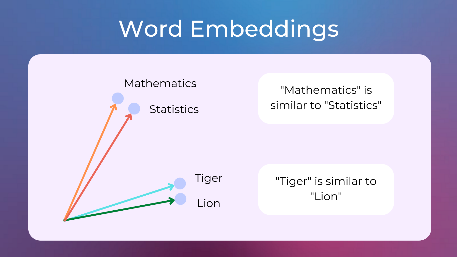
Word embeddings are a type of word representation (with numerical vectors) that allows words with similar meanings to have a similar representation.

These vectors can be learned by a variety of machine learning algorithms and large datasets of texts. One of the main roles of word embeddings is to provide input features for downstream tasks like text classification and information retrieval.

Several word embedding methods have been proposed in the past decade, here are some of them.

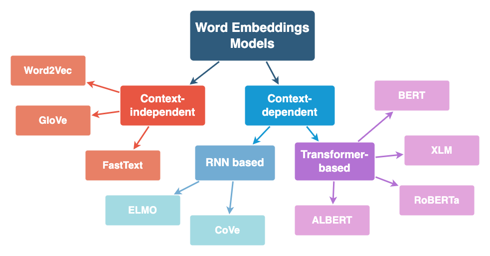
They can be split into context-independent and context-dependent embeddings. The following sections give a brief overview of different word embedding models. I’ll be using some terms that will be explained in future lessons, so don’t worry if you don’t understand everything. Try to develop an intuition of the models and I recommend giving the references a quick read.

Context-independent Embeddings

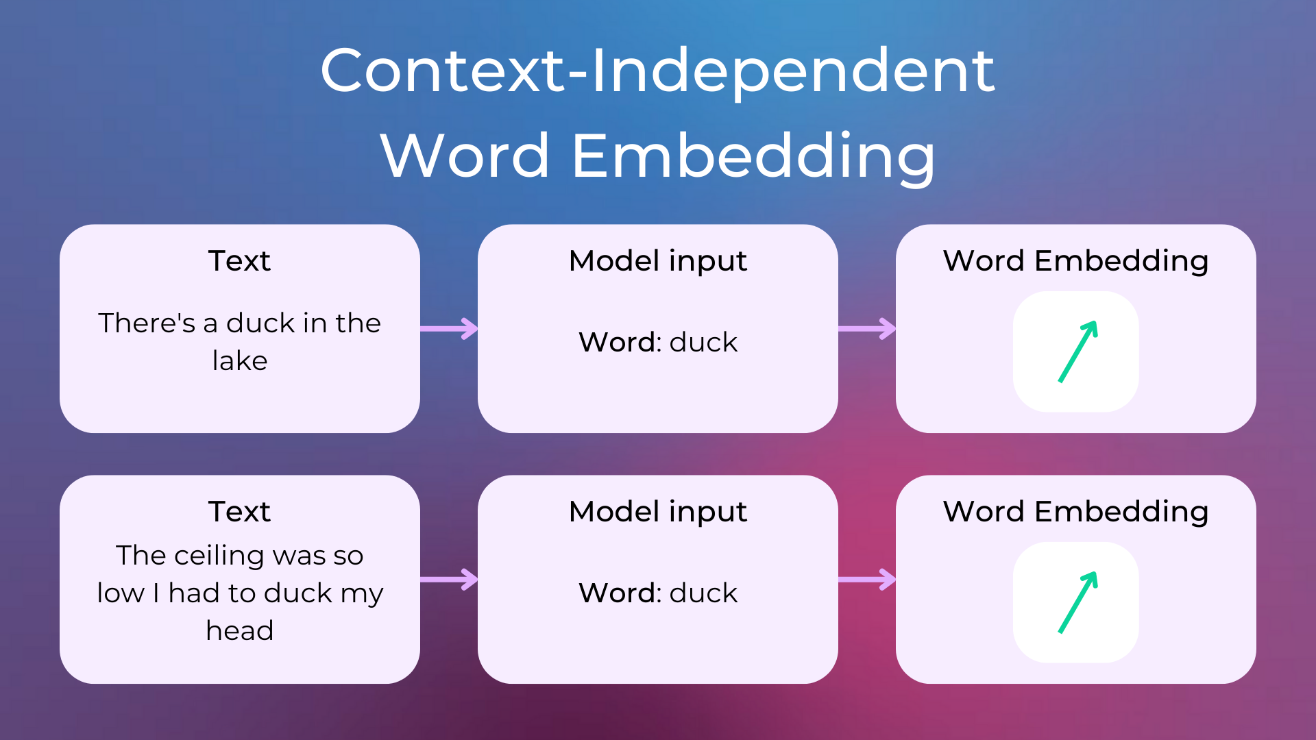
With context-independent embeddings models, the learned representations are characterized by being unique and distinct for each word, without considering the word’s context. This means that homonyms like “duck” (which can be the animal or a verb) won’t be disambiguated by their context (i.e. the text in which the word appears) and will always have a unique word embedding that somehow captures both meanings.

As a result, these models produce a map between all the words in the vocabulary and their vectors.

Here are some common context-independent embeddings:

• Word2Vec: The embeddings are learned by an algorithm involving a two-layer neural network trying to reconstruct linguistic contexts of words (so, the embeddings are learned as a side effect of the training process). Word2vec can utilize either of two model architectures: continuous bag-of-words (CBOW) or continuous skip-gram. In the CBOW architecture, the model predicts the current word from a window of surrounding context words. In the continuous skip-gram architecture, the model uses the current word to predict the surrounding window of context words.

• GloVe (Global Vectors for Word Representation): Training is performed on aggregated global word-word co-occurrence statistics from a corpus, and the resulting representations showcase interesting linear substructures of the word vector space.

• FastText: Unlike GloVe, it embeds words by treating each word as being composed of character n-grams instead of a word whole. This feature enables it not only to learn rare words but also out-of-vocabulary words.

Context-dependent Embeddings

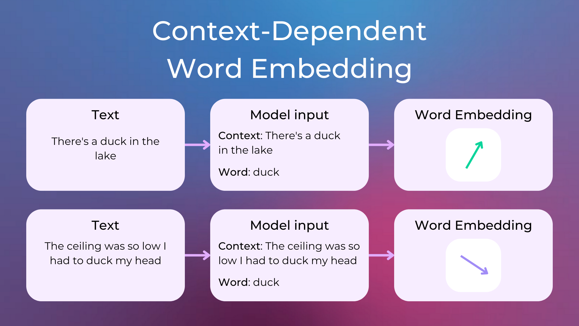
Unlike context-independent word embeddings, context-dependent methods learn different embeddings for the same word based on its context.

Context-dependent and RNN based

• ELMO (Embeddings from Language Model): Learns contextualized word representations based on a neural language model with a character-based encoding layer and two BiLSTM layers.

• CoVe (Contextualized Word Vectors): Uses a deep LSTM encoder from an attentional sequence-to-sequence model trained for machine translation to contextualize word vectors.

Context-dependent and Transformer-based

• BERT (Bidirectional Encoder Representations from Transformers): Transformer-based language representation model trained on a large cross-domain corpus. Applies a masked language model to predict words that are randomly masked in a sequence, and this is followed by a next-sentence-prediction task for learning the associations between sentences.

• XLM (Cross-lingual Language Model): It’s a transformer pre-trained using next token prediction, a BERT-like masked language modeling objective, and a translation objective.

• RoBERTa (Robustly Optimized BERT Pretraining Approach): It builds on BERT and modifies key hyperparameters, removing the next-sentence pretraining objective and training with much larger mini-batches and learning rates.

• ALBERT (A Lite BERT for Self-supervised Learning of Language Representations): It presents parameter-reduction techniques to lower memory consumption and increase the training speed of BERT.

Pre-trained Models and Finetuning

While the CountVectorizer and TfidfVectorizer must be fit from scratch every time, word embedding models can be trained once on a large corpus (maybe with an expensive but one-time training phase) and then reused without further training for most use cases, especially if the texts encoutered are similar to the ones found during training. For these reasons, there are several open-source trained word embedding models available (check the Hugging Face Hub) that everyone can use. These models are typically called pre-trained models.

Sometimes you may want to use a pre-trained embedding model on texts different from the ones encountered during pre-training, for example for classifying scientific litterature. In such case, you can often obtain better results by performing a second training phase on a more in-scope dataset. This second training phase is typically called finetuning, and the resulting model is called finetuned model.

Sentence Embeddings

Word embedding models are usually able to produce embeddings for single words. As a consequence, heuristics have been developed to get an embedding representation of a sentence or a full text, such as averaging the vectors of the words composing the sentence.

More advanced models can produce both word or sentence embeddings, such as the Sentence Transformers models. Let’s quickly see how to use the sentence_transformers library, as we’ll use it in a lot of subsequent lessons and projects.

Sentence Transformers in Python

Let’s install the sentence_transformers library.

pip install sentence-transformers huggingface-hub

We can then download one of the available sentence embeddings models, such as all-MiniLM-L6-v2, and instantiate a model.

from sentence_transformers import SentenceTransformer, util

model = SentenceTransformer('all-MiniLM-L6-v2')

Then, let’s use model.encode to compute an embedding (i.e. a numerical vector) for each of the sample sentences. The resulting vectors have 384 dimensions. Each embedding model produces embeddings of potentially different dimensions, typically from few hundreds to few thousands of dimensions.

sentences = [
    "Some kids are playing soccer",
    "There's a football match over there",
    "The house is red"
]

# compute embedding
embeddings = model.encode(sentences, convert_to_tensor=True)
print(embeddings.shape)

torch.Size([3, 384])

Last, let’s use the util.cos_sim utility function to compute the cosine similarity between pairs of embeddings.

similarity_0_1 = util.cos_sim(embeddings[0], embeddings[1])[0].item()
print(f"Sentence 0: {sentences[0]}")
print(f"Sentence 1: {sentences[1]}")
print(f"Similarity: {similarity_0_1}")
print()

similarity_0_2 = util.cos_sim(embeddings[0], embeddings[2])[0].item()
print(f"Sentence 0: {sentences[0]}")
print(f"Sentence 2: {sentences[2]}")
print(f"Similarity: {similarity_0_2}")

Sentence 0: Some kids are playing soccer
Sentence 1: There's a football match over there
Similarity: 0.21995750069618225

Sentence 0: Some kids are playing soccer
Sentence 2: The house is red
Similarity: -0.04555266350507736

Cosine similarity can have values from -1 (indicating vectors with opposite directions, and thus sentences with very different meanings) to +1 (indicating sentences with similar meanings). In this example, the two sentences about sport have a cosine similarity of 0.219, while a sentence about sport and the sentence about the colored house have a cosine similarity of -0.045.

Embeddings from different models

Each model has different training procedures and training datasets, therefore the produced embeddings may differ in quality. Indeed, there isn’t a single embedding model that is better than the others in all tasks.

MTEB is a massive benchmark for measuring the performance of text embedding models on diverse embedding tasks. Check the article to learn about the latest models and what advantages (and disadvantages) they have over other models.

What Can Be Deduced when Two Embeddings Are Similar?

In this article I said that, when two sentences have similar embeddings, they are semantically similar, but what it means exactly? Let’s make a couple of examples.

sentences = [
    "White",
    "Red"
]

embeddings = model.encode(sentences, convert_to_tensor=True)
print(util.cos_sim(*embeddings)[0].item())

0.6289807558059692

White and Red are both colors, but they are different colors. The model gives them a cosine similarity of 0.628, which is very high.

sentences = [
    "Some kids are playing soccer",
    "Some kids are not playing soccer",
]

embeddings = model.encode(sentences, convert_to_tensor=True)
print(util.cos_sim(*embeddings)[0].item())

0.8316699266433716

The two sentences are about two opposite facts: in the first one the kids are playing soccer, and in the second they aren’t. Still, their two embeddings have a high similarity, why?

The reason is in the way the embedding models are trained: indeed, they are trained to give a similar representation to words/sentences in similar contexts. For example, considering the two training sentences “I want a white shirt” and “I want a red shirt”, these models would learn to give a similar representation to the words “white” and “red” because, in the training data, they appear with the same context (i.e. the “I want a ___ shirt” sentence).

So, we can interpret a high cosine similarity between two words as a high probability for the two words of appearing in similar contexts.

Let’s Visualize Embeddings

To get a better intuition of what sentence embeddings are, let’s make a scatter plot showing the vectors of different Medium articles. Let’s import the necessary libraries.

from huggingface_hub import hf_hub_download
from sentence_transformers import SentenceTransformer, util
import pandas as pd
import numpy as np

from sklearn.decomposition import PCA # dimensionality reduction
from sklearn.manifold import TSNE # algorithm to visualize high-dimensional data

# visualization
import plotly.express as px
import plotly.io as pio

To visualize the embeddings, we’ll first reduce their dimensionality using PCA, then reduce it again to two dimensions using TSNE, and last visualize them using plotly. Both algorithms are already implemented in the sklearn library.

We download the Medium dataset and keep a subset of 200 articles about data science and 200 articles about business.

# download dataset of Medium articles from 
# https://huggingface.co/datasets/fabiochiu/medium-articles
df_articles = pd.read_csv(
  hf_hub_download("fabiochiu/medium-articles", repo_type="dataset", filename="medium_articles.csv")
)

# keep 200 articles about Data Science and 200 articles about Business
df_articles = pd.concat([
    df_articles[df_articles["tags"].apply(lambda taglist: "Data Science" in taglist)][:200],
    df_articles[df_articles["tags"].apply(lambda taglist: "Business" in taglist)][:200]
]).reset_index(drop=True)

df_articles.head()

	title	text	url	authors	timestamp	tags
0	Essential OpenCV Functions to Get You Started ...	Reading, writing and displaying images\n\nBefo...	https://towardsdatascience.com/essential-openc...	['Juan Cruz Martinez']	2020-06-12 16:03:06.663000+00:00	['Artificial Intelligence', 'Python', 'Compute...
1	Data Science for Startups: R -> Python	Source: Yuri_B at pixabay.com\n\nOne of the pi...	https://towardsdatascience.com/data-science-fo...	['Ben Weber']	2018-06-11 20:58:09.414000+00:00	['Startup', 'Python', 'Data Science', 'Towards...
2	How to Customize QuickSight Dashboards for Use...	We have been getting a lot of queries on how t...	https://medium.com/zenofai/how-to-customize-qu...	['Engineering Zenofai']	2019-12-04 11:46:34.298000+00:00	['Analytics', 'AWS', 'Big Data', 'Data Science...
3	The answer is blowing in the wind: Harnessing ...	By Glenn Fung, American Family Insurance data ...	https://medium.com/amfam/the-answer-is-blowing...	['American Family Insurance']	2020-06-12 16:41:36.697000+00:00	['Machine Learning', 'Data Science', 'AI', 'Ar...
4	Working Together to Build a Big Data Future	To leverage Big Data and build an effective Ar...	https://medium.com/edtech-trends/working-toget...	['Alice Bonasio']	2017-11-15 11:12:51.254000+00:00	['Fintech', 'Artificial Intelligence', 'AI', '...

Then, we download a sentence embeddings model.

# download the sentence embeddings model
model = SentenceTransformer('all-MiniLM-L6-v2')

Let’s concatenate titles and texts of the articles, and then compute the embedding of each article.

# concatenate title and text of articles
df_articles["full_text"] = df_articles["title"] + " " + df_articles["text"]

# compute embedding
embeddings = model.encode(df_articles["full_text"].values, convert_to_tensor=True)
print(embeddings.shape)

torch.Size([400, 384])

Next, we reduce the dimensionality of the embeddings from 384 to 2 using both PCA and TSNE.

# reduce from 384 to 50 dimensions (fast)
embeddings_pca = PCA(n_components=50).fit_transform(embeddings)

# reduce from 50 dimensions to 2 dimensions (slow, but good for visualization)
embeddings_tsne = TSNE(n_components=2, perplexity=6.0).fit_transform(embeddings_pca)

Last, let’s use plotly to create a scatter plot of the resulting 2-d vectors.

# comment the following line if you are executing on Colab
pio.renderers.default = "plotly_mimetype+notebook_connected"

# prepare data to plot
xs_tsne, ys_tsne = list(zip(*embeddings_tsne))
titles = df_articles["title"].values

# plot
df_tsne = pd.DataFrame(data={
    "x": xs_tsne,
    "y": ys_tsne,
    "title": titles,
    "color": ["color" for _ in xs_tsne]
})
labels = {
    "x": "",
    "y": "",
    "color": ""
}
hover_data = {
    "x": False,
    "y": False,
    "color": False
}
color_discrete_map = {
    "color": [
        px.colors.qualitative.Plotly[5] # light blue
        if i < len(xs_tsne) / 2
        else px.colors.qualitative.Plotly[1] # red
        for i in range(len(xs_tsne))
    ]
}
title = "Articles about Data Science (light blue) and Business (red)"
fig = px.scatter(df_tsne, x="x", y="y", hover_name="title", labels=labels, hover_data=hover_data,
                 color="color", color_discrete_map=color_discrete_map, height=400,
                 template="plotly_dark", title=title)
fig.update_xaxes(showticklabels=False)
fig.update_yaxes(showticklabels=False)
fig.update_xaxes(zeroline=False)
fig.update_yaxes(zeroline=False)
fig.update_layout(showlegend=False)
fig.update_layout({
    "plot_bgcolor": "rgba(0, 0, 0, 0)",
    "paper_bgcolor": "rgba(0, 0, 0, 0)"
})
fig.show()

Explore the scatter plot, seeing whether articles with titles about similar topics appear near each other. Observe that articles about data science distribute differently from articles about business.

Bag of Words vs Embeddings: Pros and Cons

Here’s a small list of differences between the two approaches:

• Bag of Words approaches (e.g. with CountVectorizer or TfidfVectorizer) must be fit on a training set. Instead, we can use pre-training embedding models without having to deal with training for most use cases (especially if the use case involves text similar to the texts used in the pre-training phase).

• Word embeddings models can be fine-tuned on a specific dataset, while being pre-trained on a large separate dataset (and with a more expensive pre-training phase).

• Context-dependent embeddings can disambiguate homonyms by producing different embeddings, while bag of words approaches typically can’t. As a result, context-dependent embeddings are especially better at classifying short texts (i.e. where word sense disambiguation is more important).

• Producing embeddings from a neural model is slower than using a vectorizer and may require GPUs to achieve low latencies.

Code Exercises

Go to Notebook

Quiz

What are word embeddings?

1. A type of word representation with numerical vectors that allows words with similar meanings to have a similar representation.

2. A vectorized representation of words obtained with one-hot encoding

3. A type of word representation with sparse word vectors that allows words with similar meanings to have a similar representation.

Answer

The correct answer is 1.

What is a common distinction between word embedding models?

1. Context-dependent and context-independent word embeddings.

2. Numerical and word-based embeddings.

3. Attention-dependent and attention-independent word embeddings.

Answer

The correct answer is 1.

Choose the option that better describes the ELMO and CoVe models.

1. Context-independent word embeddings.

2. Context-dependent and RNN-based word embeddings.

3. Context-dependent and Transformer-based word embeddings.

Answer

The correct answer is 2.

Choose the option that better describes the Word2Vec, GloVe and FastText models.

1. Context-independent word embeddings.

2. Context-dependent and RNN-based word embeddings.

3. Context-dependent and Transformer-based word embeddings.

Answer

The correct answer is 1.

Choose the option that better describes the BERT, XLM, RoBERTa and ALBERT models.

1. Context-independent word embeddings.

2. Context-dependent and RNN-based word embeddings.

3. Context-dependent and Transformer-based word embeddings.

Answer

The correct answer is 3.

Choose the correct option.

1. Word embeddings models are often finetuned models that can be retrained for specific use cases.

2. Word embeddings models must be trained from scratch for each specific use case.

3. Word embeddings models are often pre-trained models that can be finetuned for specific use cases.

Answer

The correct answer is 3.

Choose the correct option.

1. Sentence embeddings models compute an embedding representation of a sentence by averaging the vectors of the words composing the sentence.

2. Sentence embeddings models can compute an embedding representation of both individual words and sentences out of the box.

Answer

The correct answer is 2.

Choose the correct option.

1. The latest embedding models are always better than the previous ones in all the tasks.

2. When choosing an embedding model, it’s better to look at benchmarks to find the best ones for your specific task.

Answer

The correct answer is 2.

Questions and Feedbacks

Have questions about this lesson? Would you like to exchange ideas? Or would you like to point out something that needs to be corrected? Join the NLPlanet Discord server and interact with the community! There’s a specific channel for this course called practical-nlp-nlplanet.